RF Power Amplifier Nonlinearity Explained: Causes, Effects, Measurement…

In an ideal power amplifier, the output signal should be an amplified version of the input signal. The output waveform should have the same shape as the input waveform, with only its amplitude increased. However, real-world amplifiers cannot achieve perfect linear amplification. Various factors can cause the output waveform to differ from the input waveform. This deviation is known as amplifier distortion.

Amplifier distortion can be classified into two main types: frequency distortion (linear distortion) and waveform distortion (nonlinear distortion). Frequency distortion occurs when an amplifier provides different gain or phase delay for different frequency components of the input signal. In contrast, nonlinear distortion occurs when the output signal is no longer linearly proportional to the input signal, even at the same frequency.

These two types of distortion appear differently in signal analysis. Frequency distortion is reflected as changes in the signal spectrum in the frequency domain. Nonlinear distortion, on the other hand, is observed as waveform distortion in the time domain and the generation of additional frequency components in the frequency domain.

Compared with frequency distortion, nonlinear distortion has a greater impact on RF power amplifier performance. It generates unwanted harmonics and intermodulation products that can degrade signal quality and cause adjacent channel interference. In the following sections, we focus on the distortion of RF power amplifier nonlinearity.

Nonlinear Characteristics

From the small-signal model and input characteristic curves of an ideal transistor, you can see that a transistor amplifier itself isn’t a perfectly linear device. Plus, parasitic parameters make its linearity worse. But within a certain power range, you can treat the transistor as a linear amplifier. For power amplifier designers, the key is figuring out how to get higher output power while improving linearity.

For a transistor amplifier, its voltage-current characteristics can be described as follows:

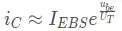
Power series expansion can be used to describe the current-voltage characteristics of a device:

In the formula, n (n=0,1,2,3,…) is a coefficient related to the characteristics of the circuit. Usually, the bigger n is, the smaller the value of the coefficient an. When the nonlinear components in the circuit are represented by a power series, the number of terms used totally depends on the signal’s amplitude and the accuracy needed.

The Impact of RF Power Amplifier Nonlinear Characteristics

The nonlinear characteristics of a device can affect an power amplifier in two ways. One is when there’s just a single signal at the input, and the other is when there’s the main signal along with one or two other signals at the input.

Input

The end only has one signal input. The signal at the input end is, substituting into formula 2, at this point we have

When the input signal has a large amplitude and the effect of the cubic term must be considered, the fundamental frequency signal obtained from formula 2 is:

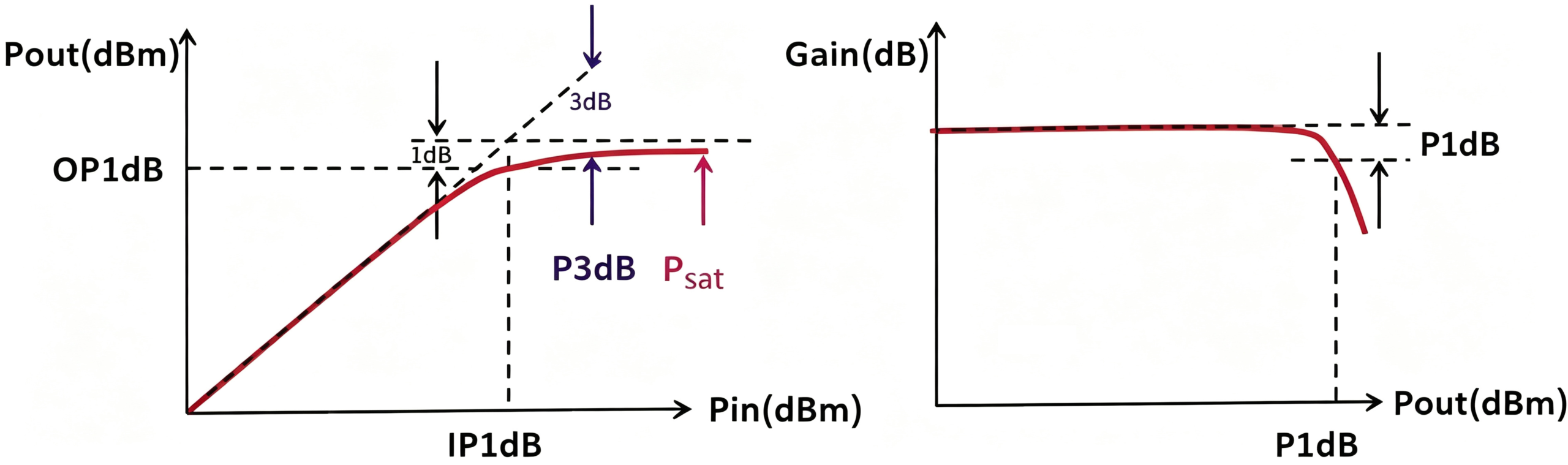
In formula 3, A3 is usually negative, which means y1(t) decreases as the input signal amplitude increases. This phenomenon is called gain compression.

The ‘1dB compression point’ is usually used in engineering to measure a device’s linear performance. The 1dB compression point is defined as the input signal power P1dB that causes the linear gain to drop by 1dB, as shown in Figure 5. Based on the definition of the 1dB compression point and equation 3, we can get

There are Two Signals at the Input

The signal amplified at the input of an amplifier is usually not a single-tone signal, but a spectrum signal composed of a certain bandwidth. Due to the nonlinearity of the device, a large number of combination interference frequency components, apart from the useful signal, can appear at the output. In addition, the combination frequency components of two or more interference signals can also interfere with the useful signal. Here’s an assumption:

Plug into formula 1，the fundamental frequency components of ω1 and ω2 are generated by the first-order and third-order terms.

A total of multiple frequency components are generated: ω1, ω2, ω1 ± ω2, 2ω1 – ω2, 2ω2 – ω1, 3ω1 – 2ω2, and 3ω2 – 2ω1.

The difference frequencies in the combination frequencies, 2ω1 – ω2 and 2ω2 – ω1, are produced by cubic terms. These two combined signal frequencies happen to fall within the sideband range of the signal frequency and could interfere with adjacent channels, making them one of the main indicators for transmission signals.

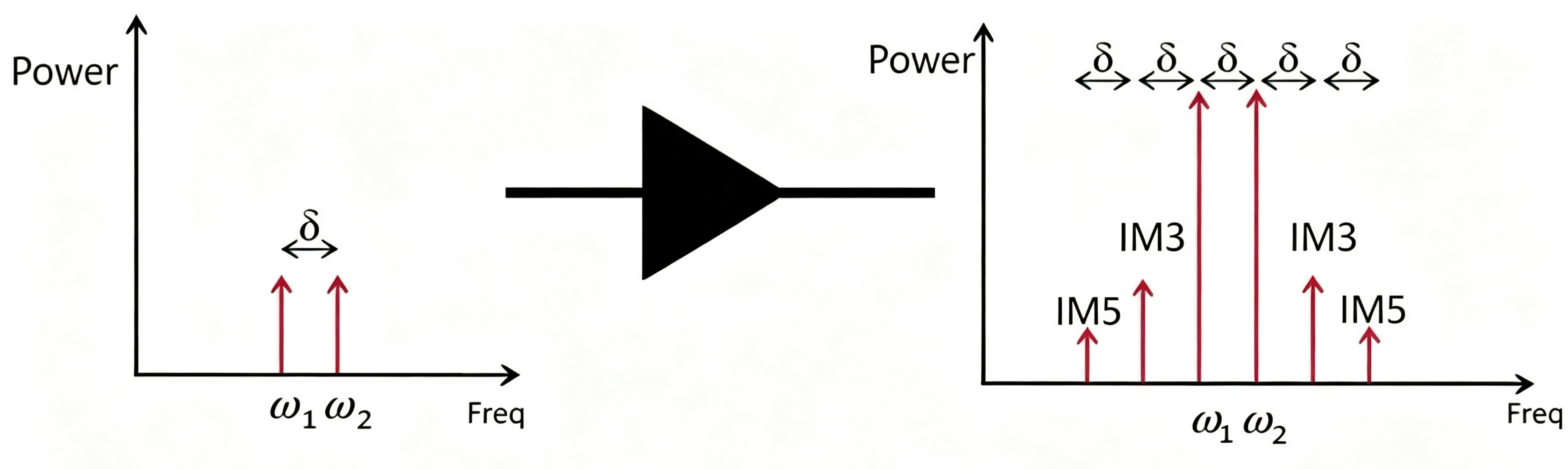
This kind of interference is caused by the mutual modulation of two signals, so it’s called intermodulation interference. At the same time, it’s generated by the cubic term, so in engineering it’s also called third-order intermodulation interference.

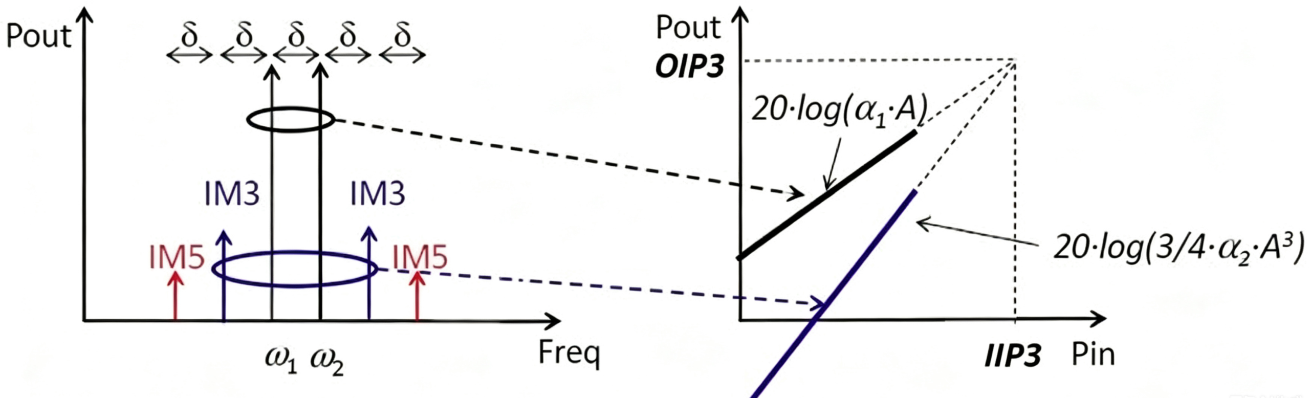
When third-order intermodulation interference is an important indicator for communication devices, engineers often use Intermodulation Distortion Ratio (IMR) and Third-Order Intercept Point (IP3) to measure it. IMR is defined as the ratio of the amplitude of the third-order intermodulation product to the amplitude of the fundamental signal at a specific input. The definition of IP3 is: when the third-order intermodulation component increases to equal the fundamental component, the receiver cannot operate normally, hence it appears.

Sideband Signal

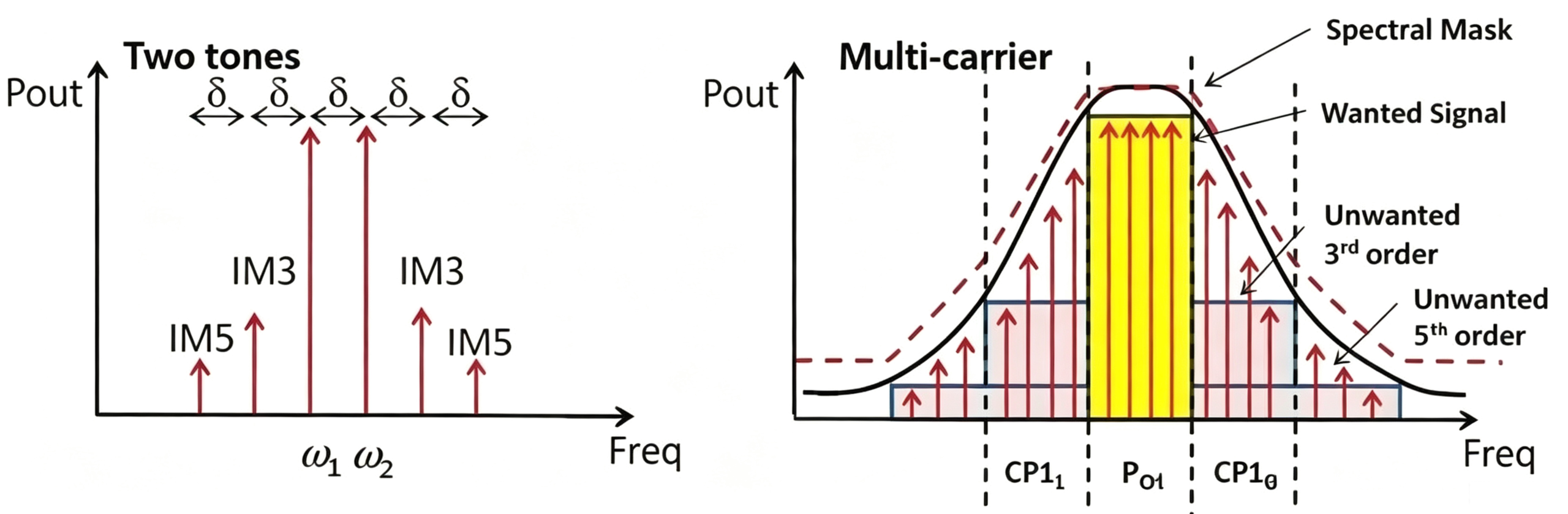
In practice, most sideband signals are generated by the intermodulation of useful signals at different frequencies within the operating bandwidth. As the input power increases, these sideband signals grow faster than the desired in-band signals. As a result, the spectrum mask gradually becomes flatter, as shown in the figure above.

Higher sideband levels can cause interference to adjacent channels and degrade overall communication performance. To minimize this interference, the IEEE 802.11 standard defines strict spectral mask requirements, as illustrated in the figure below.

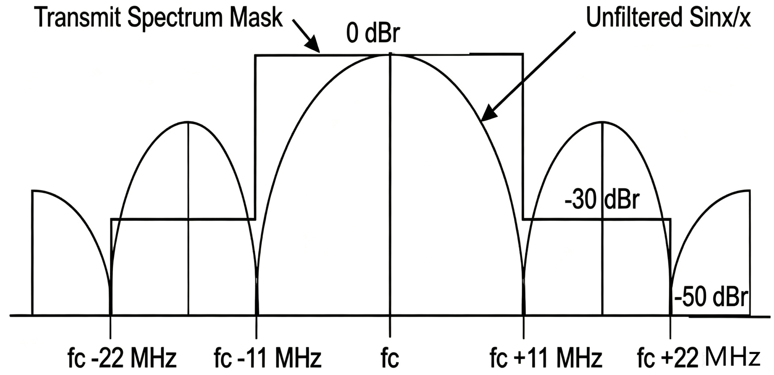
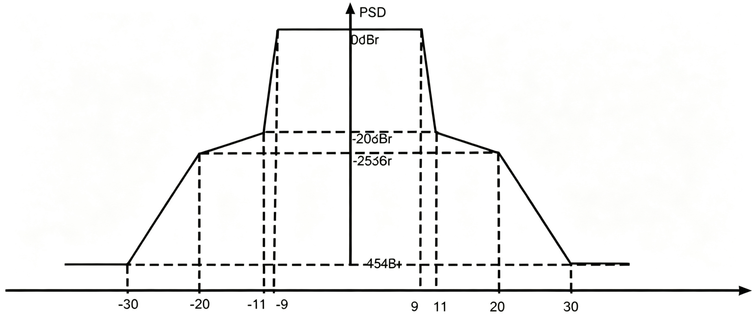
For power amplifiers, their nonlinear characteristics can increase the sidebands of a modulated signal, and the sideband amplitude is not easily suppressed by filters or other networks, which can make design tricky. So, when choosing a PA, you not only need to pay attention to its maximum linear output, but also whether it can meet the sideband spectrum requirements at that output power.

Conclusion

RF power amplifier nonlinearity is one of the most critical factors affecting wireless communication performance. It leads to gain compression, harmonic distortion, intermodulation products, and unwanted sideband emissions, all of which can reduce signal quality and cause adjacent channel interference. Understanding key parameters such as P1dB, IMD, IP3, and spectral mask is essential for designing high-performance RF power amplifiers.

By carefully selecting amplifier technologies and optimizing circuit design, engineers can improve linearity while maintaining the required output power and efficiency. This balance is increasingly important for modern applications such as 5G, satellite communications, radar, Wi-Fi, and electronic warfare.

Looking for high-performance RF power amplifiers or custom RF solutions? Contact ZR Hi-Tech. Our experienced engineering team can help you select or develop RF amplifier solutions that deliver excellent linearity, efficiency, and reliability for your specific application.